Non-Reacting CO\(_2\) Channel Flow

Description

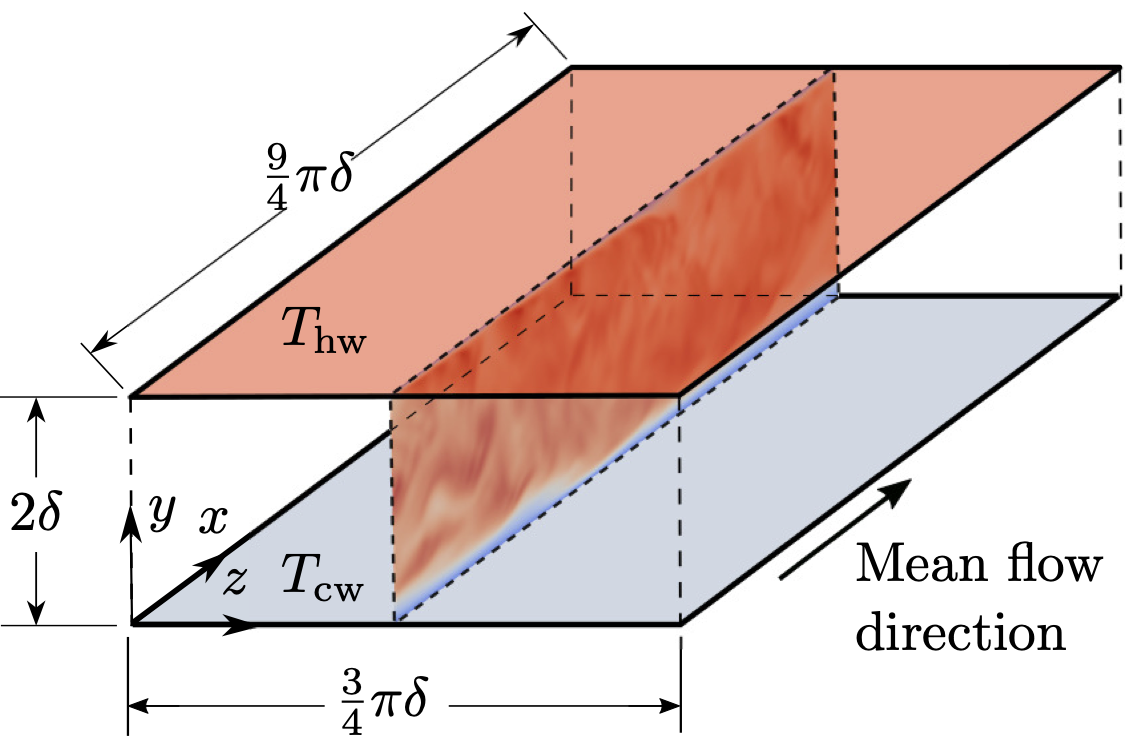
The DNS configurations in this work are part of a dataset of fully-developed high-pressure transcritical turbulent channel flow simulations using carbon dioxide (CO2) as the working fluid. The working-fluid choice is based on its well-characterized supercritical behavior, with a critical pressure of \(P_c = 7.4 MPa\) and a critical temperature of \(T_c = 304.1 K\). All simulations are conducted at supercritical bulk pressures of \(P_b/P_c = 1.5, 2.0, \text{ and } 5.0\), with subscript b indicating bulk values, spanning a range of thermodynamic conditions that traverse the pseudo-boiling region. The channel geometry consists of two isothermal walls, a cold wall (\(cw\)) and a hot wall (\(hw\)), separated by a distance of \(H = 2\delta\), with \(\delta = 175 \mu m\) denoting the channel half-height. Wall temperatures are varied such that \(T_{cw}/T_c = 0.8–0.95\) and \(T_{hw}/T_c = 1.1–1.4\), providing two temperature setups for every reduced-pressure. This thermal configuration induces a transcritical thermodynamic trajectory across the channel height, crossing the pseudo-boiling region and leading to significant property gradients and nonlinear fluid behavior. The flow is driven in the streamwise direction by imposing a bulk velocity of \(U_b = 1.0 m/s\), maintained via a proportional feedback controller (gain \(k_p = 0.1\)), which keeps relative errors below \(0.5%\). Across cases A to E, the Reynolds numbers based on bulk properties result in \(Re_b ∈ [1460, 2120]\), while the bulk Prandtl numbers span \(Pr_b \in [1.41, 2.68]\). The flow remains at low-Mach-number conditions, with bulk Mach numbers in the narrow interval \(Ma_b \in [1.7 \times 10^{−3}, 3.0 \times 10^{−3}]\). The dataset comprises six cases with snapshots of \(\rho, u, v, w, P, T, \mu, \kappa, \text{ and } c_P\) over 15 flow-through times (FTTs), once statistical stationarity is reached, resulting in 50 three-dimensional snapshots per FTT.

The computational domain is \((9/4)\pi\delta × 2\delta × (3/4)\pi\delta\) in the streamwise (x), wall-normal (y), and spanwise (z) directions, respectively. In order to accurately capture the larger streamwise and spanwise turbulent structures, the domain is set to be bigger than the minimal flow unit (MFU) configuration proposed by El Mansy et al [1]. The streamwise and spanwise boundaries are set to be periodic, and no-slip conditions are imposed on the horizontal boundaries (XZ planes). The spatial discretization employs a grid of \(96 \times 128 \times 96\) points, supplemented with two ghost cells in each direction to enable the extrapolation extrapolation of wall quantities. The grid-arrangement achieves a wall-normal distance to the first grid point away from the wall satisfying \(y^{+}_{hw} < 1.3\) and \(y^{+}_{cw} < 0.86\), which ensures adequate resolution in both boundary layers. Moreover, streamwise and spanwise resolutions satisfy \(\Delta x^{+}_{cw} \leq 8.23\), \(\Delta z^{+}_{cw} \leq 2.74\), \(\Delta x^{+}_{hw} \leq 12.47\), and \(\Delta z^{+}_{hw} \leq 4.16\), in terms of both cold- and hot-wall units. The obtained mesh resolutions remain within accepted limits for high-pressure transcritical wall-bounded flows [2].

The equations of fluid motion are computationally solved using the in-house flow solver RHEA [3]. Spatial operators are treated using second-order central differencing schemes, and time-advancement is explicitly performed by means of a third-order strong-stability preserving (SSP) Runge-Kutta approach [4]. The Kennedy-Gruber-Pirozzoli (KGP) splitting is adopted for the convective terms extended to high-pressure transcritical fluids turbulence [5], ensuring kinetic-energy preservation by convection. This numerical framework provides stable computations without the need of any form of artificial dissipation or stabilization procedures. To accurately represent real-fluid behavior in the transcritical regime, thermodynamic properties are evaluated using the Peng–Robinson equation of state [6], while transport properties are determined from the correlations proposed by Chung et al. [7,8].

Quick Info

• Contributors: Reda El Mansy, Guillem Barea, Lluis Jofre

• N_ɸ = 5 + 4

• DOI
• .bib

Links to different cases

Case	$P_b/P_c$	$T_{hw}/T_c$	$T_{cw}/T_c$	Size (GB)	Links
1	1.5	1.1	0.95	32	Kaggle, info.json
2	1.5	1.2	0.90	32	Kaggle, info.json
3	1.5	1.4	0.80	32	Kaggle, info.json
4	2.0	1.1	0.95	32	Kaggle, info.json
5	2.0	1.2	0.90	35	Kaggle, info.json
6	2.0	1.4	0.80	30	Kaggle, info.json

References

[1] R. E. Mansy, C. Monteiro, F. Mellibovsky, and L. Jofre, “Minimal flow unit of wall-bounded high-pressure transcritical turbulence,” Phys. Fluids 36, 125182 (2024).
[2] C. Monteiro and L. Jofre, “Resolution standards for direct numerical simulation of wall turbulence in high-pressure transcritical fluids,” Phys. Fluids 36, 125184 (2024).
[3] L. Jofre, A. Abdellatif, and G. Oyarzun, “RHEA - an opensource Reproducible Hybrid-architecture flow solver Engineered for Academia,” J. Open Source Softw. 8, 4637 (2023).
[4] S. Gottlieb, C. W. Shu, and E. Tadmor, “Strong stability preserving high-order time discretization methods,” SIAM Review 43, 89–112 (2001).
[5] M. Bernades, L. Jofre, and F. Capuano, “Kinetic-energy- and pressure-equilibrium-preserving schemes for real-gas turbulence in the transcritical regime,” J. Comput. Physics 493, 112477 (2023).
[6] D. Y. Peng and D. B. Robinson, “A new two-constant equation of state,” Ind. Eng. Chem. Fundam. 15, 59–64 (1976).
[7] T. H. Chung, L. L. Lee, and K. E. Starling, “Applications of kinetic gas theories and multiparameter correlation for prediction of dilute gas viscosity and thermal conductivity,” Ind. Eng. Chem. Fund. 23, 8–13 (1984).
[8] T. H. Chung, M. Ajlan, L. L. Lee, and K. E. Starling, “Generalized multiparameter correlation for nonpolar and polar fluid transport properties,” Ind. Eng. Chem. Fund. 27, 671–679 (1988).